In this post we will talk briefly about the Euler-Lagrange equations and show a simple application. Consider a differentiable application $L:\mathbb{R}^n \times \mathbb{R}^n \times \mathbb{R} \rightarrow \mathbb{R}$. We will call this application an action. Now, take a curve $\gamma : [a,b] \rightarrow \mathbb{R}^n$. Consider the "inclusion" $\widetilde{\gamma}: [a,b] \rightarrow \mathbb{R}^n\times \mathbb{R}^n \times \mathbb{R}$ given by $\widetilde{\gamma}(t)=(\gamma(t), \dot{\gamma(t)}, t)$. The action of $L$ in $\gamma$ is defined as
$$A_L(\gamma):=\int_a^b L \circ \widetilde{\gamma}.$$
This defines a map $A_L: Crvs \rightarrow \mathbb{R}$, where $Crvs$ is some space of curves. We will take, for now, $Crvs$ to be the affine space $C^1([0,1], \mathbb{R}^n, p,q)$ of $C^1$ curves with initial point $p$ and endpoint $q$, with underlying vector space $C^1([0,1], \mathbb{R}^n, 0,0)$ with its $C^1$ norm. Therefore, $Crvs$ is an affine space and we can talk about derivatives here. Moreover, this is a Banach affine space, which makes the situation quite pleasant since we can not only compute derivatives (which is available in any normed space) but also solve differential equations, find extrema etc (although we are not interested in these aspects in this post). However, there are cases where other spaces are desirable and/or more convenient.

Let's find the critical points of $A_L$. Fix $\gamma \in Crvs$. Note that
$$\big(L \circ (\widetilde{\gamma + h})\big)(t)=L\big( \gamma(t)+h(t), \dot{\gamma}(t)+\dot{h}(t), t \big) $$
$$=L \big( \gamma(t), \dot{\gamma}(t), t \big)+L'_{(\gamma(t),\cdot{\gamma(t)},t)} \cdot \big( h(t), \dot{h}(t), 0 \big) + \epsilon\big(h(t), \dot{h}(t), 0 \big) $$
$$=L \big( \gamma(t), \dot{\gamma}(t), t \big)+\nabla_1 L_{(\gamma(t),\cdot{\gamma(t)},t)} \cdot \big( h(t) \big) $$
$$ +\nabla_2 L_{(\gamma(t),\cdot{\gamma(t)},t)} \cdot \big( \dot{h}(t) \big) + \epsilon\big(h(t), \dot{h}(t), 0 \big)$$
$$=L \big( \gamma(t), \dot{\gamma}(t), t \big)+\nabla_1 L_{(\gamma(t),\cdot{\gamma(t)},t)} \cdot \big( h(t) \big)$$ 
$$ +\dot{\bigg(\nabla_2 L_{(\gamma(t),\cdot{\gamma(t)},t)} \cdot \big( h(t) \big)\bigg)} -\dot{\bigg(\nabla_2 L_{(\gamma(t),\cdot{\gamma(t)},t)}} \bigg) \cdot \big( h(t) \big) + \epsilon\big(h(t), \dot{h}(t), 0 \big),$$
where $\nabla_1$ are the first $n$ components of the gradient of $L$, and $\nabla_2$ are the next $n$ components. Hence, we have that
$$A_L(\gamma+h)=\int_a^b \big[L \big( \gamma(t), \dot{\gamma}(t), t \big)+\nabla_1 L_{(\gamma(t),\cdot{\gamma(t)},t)} \cdot \big( h(t) \big)$$ 
$$ +\dot{\bigg(\nabla_2 L_{(\gamma(t),\cdot{\gamma(t)},t)} \cdot \big( h(t) \big)\bigg)} -\dot{\bigg(\nabla_2 L_{(\gamma(t),\cdot{\gamma(t)},t)}} \bigg) \cdot \big( h(t) \big) + \epsilon\big(h(t), \dot{h}(t), 0 \big) \big]dt$$ 
$$=A_L(\gamma)+ \bigg(\nabla_2 L_{(\gamma(t),\cdot{\gamma(t)},t)} \cdot \big( h(t) \big)\bigg) \bigg|_a^b $$
$$+\int_a^b \big[ \nabla_1 L_{(\gamma(t),\cdot{\gamma(t)},t)} \cdot \big( h(t) \big) - \dot{\bigg(\nabla_2 L_{(\gamma(t),\cdot{\gamma(t)},t)}} \bigg) \cdot \big( h(t) \big) \big]dt$$ 
$$+ \int_a^b \epsilon\big(h(t), \dot{h}(t), 0 \big)dt $$
$$=A_L(\gamma)$$
$$+\int_a^b \big[ \nabla_1 L_{(\gamma(t),\cdot{\gamma(t)},t)} \cdot \big( h(t) \big) - \dot{\bigg(\nabla_2 L_{(\gamma(t),\cdot{\gamma(t)},t)}} \bigg) \cdot \big( h(t) \big) \big]dt$$ 
$$+ \int_a^b \epsilon\big(h(t), \dot{h}(t), 0 \big)dt $$
The Lebesgue Dominated Convergence Theorem (or uniform convergence on compact sets of the error of a differential) can then be used to conclude that
$$(D_{\gamma}A_L)( h ) = \int_a^b \big[ \nabla_1 L_{(\gamma(t),\cdot{\gamma(t)},t)} \cdot \big( h(t) \big) - \dot{\bigg(\nabla_2 L_{(\gamma(t),\cdot{\gamma(t)},t)}} \bigg) \cdot \big( h(t) \big) \big]dt.$$
We then have that $D_{\gamma} A_L=0$ (that is, it is the $0$ functional) if and only if
$$ \nabla_1 L_{(\gamma(t),\cdot{\gamma(t)},t)} - \dot{\bigg(\nabla_2 L_{(\gamma(t),\cdot{\gamma(t)},t)}} \bigg) \equiv 0.$$
The above equation is called the Euler-Lagrange equation.

We will now present a simple application. Consider the action $L: \mathbb{R}^2 \times \mathbb{R}^2 \times \mathbb{R} \rightarrow \mathbb{R}$ given by
$$L(x,y,t)=\|y\|^2.$$
Note that the action of $L$ on a path will yield its energy. We compute $\nabla_1$ and $\nabla_2$:
$$\nabla_1 L(x,y,t)=0,$$
$$\nabla_2 L(x,y,t)=2y.$$
Therefore,
$$\nabla_1 L_{(\gamma(t),\cdot{\gamma(t)},t)}=0,$$
$$\nabla_2 L_{(\gamma(t),\cdot{\gamma(t)},t)}=2\dot{\gamma}(t)$$
The Euler-Lagrange equation then tells us that the extremal path satisfies
$$ \nabla_1 L_{(\gamma(t),\cdot{\gamma(t)},t)} - \dot{\bigg(\nabla_2 L_{(\gamma(t),\cdot{\gamma(t)},t)}} \bigg) \equiv 0$$
$$\therefore 0-2\ddot{\gamma}(t)=0 \quad \forall t.$$
$$\therefore \ddot{\gamma}(t)=0 \quad \forall t,$$
which shows us that the critical paths are lines with constant velocity, which was expected.

As an ending note, we observe that, on a manifold, the action is a function $L: TM \times \mathbb{R} \rightarrow \mathbb{R}$, as expected.

When studying Linear Algebra we see the identification of matrices and linear maps between vector spaces. However, this identification is sometimes abused and/or badly understood, to the point of utter confusion. We present formally what this identification conveys. For what follows to make sense and be interpreted as the structural result it really is, we introduce some language from Category Theory. We will not add all the details. For those readers interested, we refer to the book Algebra by Serge Lang or Algebra: Chapter $0$ by Paolo Aluffi. The wikipedia entry is also sufficient for a introduction. A Category $\mathcal{C}$ is a collection of objects $\mathcal{O}$, together with a collection $Hom$ of morphisms $Hom(A,B)$ for each pair of objects $A,B \in \mathcal{O}$ , which can be thought as arrows that leave $A$ and arrive at $B$. Those arrows are required to behave like functions: for instance, there exists a composition of morphisms, for every object there exists an identity morphism etc. Just as a metric space $M$ can sometimes be represented as $(M,d)$, a category may be represented as $(\mathcal{C}, \mathcal{O}, Hom)$.

Examples of categories are ubiquitous. For instance, we have the category $\text{FVect}$ whose objects are finite-dimensional vector spaces and morphisms are linear maps, we have the category $\text{Top}$ whose objects are topological spaces and morphisms are continuous maps, we have the category $\text{ProdK}$ whose objects are finite cartesian products of a field $\mathbb{K}$ (with its canonical vector-space structure) and whose morphisms are the functions which are multiplication by matrices, etc. We note that morphisms need not be functions, and objects need not be sets. However, we will not need to discuss that for what follows. A functor between two categories $\mathcal{C}_1$ and $\mathcal{C}_2$ is an association between two categories in the following sense: it takes an object of $\mathcal{C}_1$ to an object of $\mathcal{C}_2$, and a morphism between two objects in $\mathcal{C}_1$ to a morphism between the two objects associated in $\mathcal{C}_2$. We also require that composition of morphisms is taken to composition of morphisms, and that the identity is taken to the identity. An example will come shortly.
​
Consider now the category $\text{BFVert}$, where the objects are finite-dimensional vector spaces $V$, considered together with an ordered basis $B$ (that is, the objects are $(V,B)$) and the morphisms are the linear transformations. The "identification"{} between linear transformations and matrices can now be stated as follows:

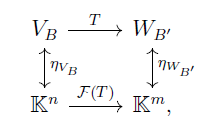
Proposition: There exists a functor $\mathcal{F}: \text{BFVert} \rightarrow \text{ProdK}$ which sends the objects $V_B$ of $\text{BFVert}$ to the space $\mathbb{K}^n$, where $n=\dim(V)$, and makes the following diagram commute:







​
​




​
​
where $\mathbb{K}^n=\mathcal{F}(V_B)$, $\mathbb{K}^m=\mathcal{F}(W_{B'})$ and $\eta_{V_B}$, $\eta_{W_B'}$ are the isomorphisms (in the vector-space sense) which take the elements of the basis and send them, orderly, to the canonical basis of $\mathbb{K}^n$ and $\mathbb{K}^m$, respectively.

Proof: The proof of this is what is done in Linear Algebra, so we leave it as exercise. $\blacksquare$ 
Note that the matrix associated to $T$ is, therefore, $\mathcal{F}(T)$. Note also that a functor satisfying such properties is unique, as easily verified by the fact that the coefficients of the matrix is imposed by the properties of the functor.

Having stated the identification between matrices and linear maps in such a clear and precise way, it eludes me how Category Theory took so long to be developed, waiting up to Algebraic Topology to force it to surface.

We end this discussion by noting that the $\eta$ isomorphisms which appear in the diagram also have a nice generalization. They constitute a natural transformation between the identity functor and the functor $\mathcal{F}$. Interested readers are invited to look up the concept.

In this post, I'll present a nice application of ordinals (specifically, transfinite induction/recursion) in order to arrive at a result of basic Real Analysis.

It is of my opinion that the Least Upper Bound axiom is a strong one, which usually has never been thought before by a student by the time he first learns it. As I've already argued before with some colleagues, having a least upper bound for any subset of $\mathbb{R}$ which is bounded by above is quite a statement. Subsets of $\mathbb{R}$ can be quite weird and difficult to handle (see, for instance, the Continuum Hypothesis).

However, it is of natural intuition that every increasing, bounded sequence of real numbers converges. This is a simple statement, and one that even a high-school student can easily understand and agree with after some thought (and maybe persuasion).

It is a basic fact of analysis that the Least Upper Bound axiom implies what we will call the Monotone Convergence Axiom for Sequences (MCAS, shortly): every increasing, bounded sequence of real numbers converges.

We will prove that MCAS implies the Least Upper Bound axiom. More precisely, we will prove that:

Theorem: If $\mathbb{R}$ is an ordered field containing the rational numbers (with its usual order) and which satisfies the MCAS, then $\mathbb{R}$ satisfies the Least Upper Bound axiom.

It is an easy consequence of MCAS that $\mathbb{R}$ satisfies the Archimedean Property, that is:

Proposition: For every $x,y>0$, there exists $n>0$ such that

$$nx>y.$$

Proof: If the proposition was false, then the sequence $nx$ would be bounded. Since it is clearly increasing, we would have that $nx \rightarrow a$ for some $a$. Note that $(n+1)x$ is a subsequence, hence we would have that $a=a+x \implies x=0$, a contradiction.

It also follows easily the density of rationals (this only uses the Archimedean Property). We leave this as an exercise.

Now, we want to prove that $\mathbb{R}$ satisfies the Least Upper Bound axiom. Therefore, take $A \subset \mathbb{R}$ bounded by above. We must prove that $A$ has a least upper bound.

A first idea would be to take an increasing sequence of elements of $A$ and hope for it to converge to what should be the least upper bound. However, this clearly is not intelligent enough, since the following situation could happen




​







One might be tempted to abandon this idea and pursue something with more finesse. However, stubbornness can also yield fruitful results. The idea is... keep doing this. Do it, and if the limit of your sequence is not a least upper bound, do it again. Then repeat and repeat etc etc. If you do this, but do it really fast, being able to jump infinite cases which prove not to be useful, you have to be right eventually.

That is the core idea. We now proceed with the proof:

Suppose $A$ has no least upper bound.

Consider the set $\Omega$ (the least uncountable ordinal. Remember that $\Omega=[0,\Omega)$). We will define a function $f: \Omega \rightarrow \mathbb{Q}$ by transfinite recursion.

Take $f(0)$ to be any rational smaller than an element of $A$.

Given $f(a)$, take $f(a+1)$ to be a rational greater than $f(a)$ and smaller than an element of $A$.

Given a limit ordinal $\gamma$, suppose we have defined an increasing function on the ordinals for all ordinals $\beta$ smaller than $\gamma$ in such a way that each $f(\beta)$ is smaller than some $b \in A$. We have that there exists an increasing sequence of ordinals $\alpha_n$ smaller than $\gamma$ that converges to the limit ordinal (order topology). The associated $f(\alpha_n)$ is a bounded increasing sequence of real numbers, hence converge to a given real number $x$. Take a rational number which is greater than $x$, and smaller than an element of $A$ (this is guaranteed by the assumption that there is no least upper bound of $A$), and make $f(\gamma)$ to be this rational number. This completes the construction of $f$. We have thus constructed an injection from $\Omega$ to $\mathbb{Q}$. But $\Omega$ isn't enumerable, so we have reached a contradiction.

 "Mathematics occurs on the boundary between the obvious and the impossible."

Since I'm tutoring Topology this semester, I thought it would be a good idea to make a post on something introductory of Topology. So, I remembered the following exercise of the very beginning of the course:

Exercise: Let $\tau$ and $\tau'$ be topologies on a set $X$. Then, the identity map $(X, \tau) \hookrightarrow (X,\tau ')$ is continuous iff $\tau' \subset \tau$.

The proof is trivial. As a corollary, one gets:

Corollary: $\tau = \tau'$ iff the identity is a homeomorphism.

All of the above are easy results that seem to be only mild exercises. We now show that they furnish a way to understand how rigid a compact hausdorff topology is.

For that, consider the following observations which follow from the definitions.

OBS1: If $(X,\tau)$ is hausdorff and $\tau \subset \tau'$, then $(X,\tau')$ is hausdorff.

OBS2: If $(X,\tau')$ is compact and $\tau \subset \tau'$, then $(X,\tau)$ is compact.

Now we present the only non-trivial lemma of this post (although it is quite straight-forward):

Lemma: Every continuous bijective function from a compact space to a hausdorff space is a homeomorphism.

Proof: It suffices to prove that image of closed sets is closed. Take a closed set on the domain. Since it is closed on a compact space, it is compact. Its image is therefore compact. But a compact set in a hausdorff space is closed. $\blacksquare$

Now we come to the crux of the post:

Proposition: Let $(X,\tau)$ be a compact hausdorff space. If $\tau' \subsetneq \tau$, then $(X,\tau')$ is not hausdorff. If $\tau' \supsetneq \tau$, then $(X,\tau')$ is not compact.
In other words, if you take off open sets of $\tau$ you lose hausdorffness and if you put new open sets in $\tau$ you lose compactness.

Proof: The reader may want to prove this on his own. If not, go ahead.

Let's prove the first case. Suppose $(X,\tau')$ is hausdorff. By OBS2, we have that $(X,\tau')$ is compact. Hence, by the exercise together with the lemma, we have that the identity is a homeomorphism. By the corollary of the exercise, this implies $\tau' =\tau$, a contradiction. Similarly, we have the second case. $\blacksquare$

This can be illustrated with as follows:

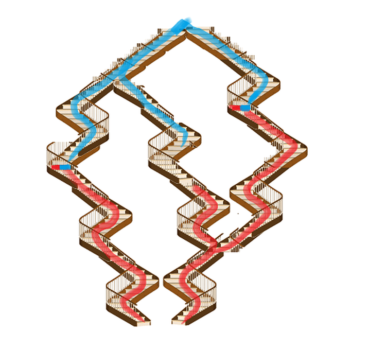
Imagine we have a flight of stairs. Each step of the stair is a topology on a given set $X$. The bottom is the trivial topology, the top is the discrete topology. A red step means a topology which makes $X$ compact, and a blue step is a topology which makes $X$ hausdorff. What the theorem above says is that in a given "line" of stairs, there can be at most one step which is both red and blue.











​

​

Let $f: \mathbb{H} \rightarrow \mathbb{R}$ be a differentiable mapping, where $\mathbb{H}$  is a banach space. Consider the segment $tx$. This way, we have a function $\tilde{f}:[0,1] \rightarrow \mathbb{R}$ given by $\tilde{f}(t)=f(tx)$.

By the fundamental theorem of calculus,

$$f(x)=f(0)+\int_0^1 \tilde{f}'(t)dt=f(0)+\int_0^1 D_{tx}f(x)dt$$

We shall demonstrate the following lemmas:

Lemma: Let

$$A: \mathbb{H} \rightarrow L(\mathbb{H},\mathbb{R})$$

$$x \mapsto A_x$$

and

$$g: \mathbb{H} \rightarrow \mathbb{H}$$

be differentiable functions. Then,

$$D_x(A(g))=A_x(D_xg(~ \cdot ~))+ (D_xA(~\cdot ~)) g(x)$$

Proof:

$$A_{x+h}(g(x+h))=(A_x+D_xA(h)+\epsilon(h))(g(x)+D_xg(h)+\xi(h))$$

$$=A_xg(x)+A_x(D_xg(h))+(D_xA(h))(g(x))+ \zeta(h)$$

where $\frac{\zeta(h)}{||h||} \rightarrow 0$


$\blacksquare$




Corollary: [Integration by Parts] Given a function $\xi :\mathbb{R} \rightarrow \mathbb{H}$ and two functions $A$, $g$ as in the previous lemma, we have:

$$A_{\xi(1)}(g(\xi(1)))-A_{\xi(0)}(g(\xi(0)))=\int_0^1 A_{\xi(t)}(D_{\xi(t)}g( \xi'(t))) dt + \int_0^1 (D_{\xi(t)}A(\xi '(t)))(g(\xi(t)))dt$$

Proof

Fundamental Theorem of Calculus.

$\blacksquare$


Corollary: Given differentiable functions:

$$A: \mathbb{H} \rightarrow L(\mathbb{H},\mathbb{R})$$

$$x \mapsto A_x$$

and

$$h: \mathbb{R} \rightarrow \mathbb{H}$$ 

,we have:

$$A_{h(1)}(h(0))-A_{h(0)}(h(1))=\int_0^1 A_{h(t)}(-h'(t)) dt + \int_0^1 (D_{h(t)}A(h '(t)))(h(1)+h(0)-h(t))dt$$

Proof:  Use $\xi=h$ and $g(z)=h(1)+h(0)-z$ in the previous corollary.

$\blacksquare$

Applying the above corollary to $h(t)=(1-t)x$ and $A=Df$, we obtain:

$$D_0f(x)-D_xf(0)=\int_0^1D_{(1-t)x}f(x)dt+\int_0^1((D_{(1-t)x}Df)(-x))(x-(1-t)x)dt$$

We then have:

$$\int_0^1D_{(1-t)x}f(x)dt =D_0f(x) -\int_0^1((D_{(1-t)x}Df)(-x))(x-(1-t)x)dt$$

Changing variables, we get:

$$\int_0^1D_{tx}f(x)dt =D_0f(x) -\int_0^1((D_{(tx)}Df)(-x))(x-tx)dt$$

$$\implies \int_0^1D_{tx}f(x)dt =D_0f(x) - \int_0^1((D_{(tx)}Df)(-x))((1-t)x)dt$$

Therefore,

$$f(x)=f(0)+D_0f(x)- \int_0^1((D_{(tx)}Df)(-x))((1-t)x)dt$$


Note that, in the above equation, we have the same hypotheses of the first lemma. This way, we can keep applying integration by parts repeatedly, obtaining:




$$f(x)=f(0)+D_0f(x)+\frac{1}{2}(D_0Df(x))(x)+...+R$$




where $R$ is an integral remainder

The extended real line, which we will soon define, is a useful setting in the study of measure and integration, for example. But, in that context, it is seen primarily as a tool, and the topological properties that one can acquire from it remains relatively shaded, since the focus is on its useful algebraic properties, and simple limit properties. We shall see that one can arrive in interesting results (that hold even when you consider problems on $\mathbb{R}$ itself) quite easily with it.

IDEA: We want to attach two points to the real line and call them $\infty$ and $-\infty$, and we want them to behave as we expect from something we would call $\infty$ and $-\infty$. For that, if we want to talk about the topology of this resulting space, we essentially have to say what are the neighbourhoods of this topology. We still want $(a-\delta,a+\delta)$ to be a neighbourhood of a real number $a$, for example. But we also want neighbourhoods of $\infty$ now. It seems a reasonable attempt to define a neighbourhood of $\infty$ as $(M,\infty]$ for example (note the closed bracket, indicating that $\infty$ is in the set).

Before proceding, I introduce the concept of a basis of a topology. Essentially, the basis of a topology is a smaller, "controlled" set that generates the topology - it says who the open sets are.

Definition: If $X$ is a set, a basis of a topology in $X$ is a collection $\mathcal{B}$ of sets that satisfy the following properties:

(i) For all $x \in X$ there is a set $B$ in $\mathcal{B}$ that contains $x$
(ii) If $x$ is in the intersection of two basis elements $B_1$ and $B_2$, then there is a basis element $B_3$ that contains $x$ and that is contained in the intersection of $B_1$ and $B_2$. 

We define the topology $\tau$ generated by $\mathcal{B}$ to be the collection of sets $A$ that satisfy the property that for all $x \in A$, there is a basis element $B$ containing $x$ and contained in $A$.

For example, the balls of a metric space are a basis for its topology (draw it in order to understand!)
Another example of a basis (which is, in fact, a corollary of the balls of metric spaces) are the open intervals in the real line.

Of course, there are technical issues (minor ones, easily solved) that I'll overpass. We have to prove that the topology generated by $\mathcal{B}$ is in fact a topology, as defined in a previous post. If you are interested, you can do it as an exercise.

Now, let's jump into what we wanted!

Definition: Take two points that are not in $\mathbb{R}$ and call them $\infty$ and $-\infty$. Now, define
$$\displaystyle \overline{\mathbb{R}}:=\mathbb{R} \cup \{\infty,-\infty\}$$
Furthermore, define the following basis on $\displaystyle \overline{\mathbb{R}}$:
The basis $\mathcal{B}$ will consist of the open intervals and of the sets $(b, \infty]$ and $[-\infty, a)$ for all $b$ and $a$ real numbers.

That this is in fact a basis (which means that this satisfies the properties listed before) is easy to verify.

Now, in order not to introduce a lot of notations and definitions, I'll not define the subspace topology. It is not a difficult definition, but may be abstract and not enlightening at first. Hence, I'll just assume an intuition in it, in order to justify the following: it seems clear that, if you have 
$\displaystyle \overline{\mathbb{R}}$ and pass from it to $\mathbb{R}$, the topology you inherit is exactly the standard topology of $\mathbb{R}$. We will use this fact.

We arrive now at a change of point of view:

In analysis, one often learns the following definition:

We say a sequence $x_n$ converges if there is a real number $L$ such that $\forall \epsilon >0$ there exists a $N \in \mathbb{N}$ such that $n > N \implies |x_n - L| < \epsilon$. In this case, we call $L= \lim x_n$. Otherwise, we say the sequence diverges.

But we also have the following definition: 

($1$) Given a sequence $x_n$, we say $\lim x_n= \infty$ if $\forall A \in \mathbb{R}$ there is a $N \in \mathbb{N}$ such that $n > N \implies x_n> A$. 



Note that this is a slight abuse of notation. The sequence $x_n$ above, BY DEFINITION, does not converge. But we say  $\lim x_n= \infty$, because it makes sense. To be completely honest, we should write something different, like $L ~x_n= \infty$

But note that, according to our topology, we have that the definition of $L ~x_n= \infty$ is in fact the definition of $\lim x_n= \infty$. In fact, ($1$) is precisely telling: For all neighbourhoods $V$ of infinity, there exists an $N$ such that $n > N \implies x_n \in V$. So, $x_n$ CONVERGES, and REALLY CONVERGES to $\infty$.

We come to our first proposition:


Proposition: $\displaystyle \overline{\mathbb{R}}$ is compact.


Proof: Take an open cover $V_i$ of $\displaystyle \overline{\mathbb{R}}$. Choose a $V_{i_1}$ such that it contains $+\infty$, and a $V_{i_2}$ such that it contains $-\infty$. They contain a set of the form $(b,\infty]$ and $[-\infty, a)$ respectively, so the rest of the $V_i$ should cover $[a,b]$, which is contained in the complement of those sets. But, by the Heine-Borel Theorem, $[a,b]$ is compact. Hence, there is a finite subcover of $V_i$ that covers $[a,b]$. So, this finite subcover, together with  $V_{i_1}$ and  $V_{i_2}$ covers $\displaystyle \overline{\mathbb{R}}$. So, we arrived at a finite subcover for $\displaystyle \overline{\mathbb{R}}$. $\blacksquare$.

Corollary: Every sequence in $\displaystyle \overline{\mathbb{R}}$ has a convergent subsequence.


Note the analogy between bolzano-weierstrass theorem and the corollary above. Bolzano-weierstrass says every bounded sequence has a convergent subsequence. 


We arrive now at a result that does not involve $\displaystyle \overline{\mathbb{R}}$ at first sight:

Proposition: Let $f:[0,\infty) \rightarrow \mathbb{R}$ be a continuous function such that $\displaystyle \lim _{x \rightarrow \infty}f(x) =L$, and $L<f(0)$. Then, $f$ has a maximum.

Proof: Define $\overline{f} :[0,\infty] \rightarrow \mathbb{R}$ as $f(x)$ if $x \in [0,\infty ) $ and $L$ if $x=\infty$. Since $\displaystyle \lim _{x \rightarrow \infty} f(x)=L$, $\overline{f}$ is continuous in $[0,\infty]$. Since $[0,\infty]$ is closed (not proved, but easily seen to be true) and $\displaystyle \overline{\mathbb{R}}$ is compact, $[0,\infty]$ is compact. Hence, $\overline{f}$ reaches a maximum on $[0,\infty]$. This maximum cannot be in $\infty$, since $f(0)>f(\infty)$. Hence, this maximum must be achieved in $[0,\infty)$. $\blacksquare$


Note somethings in the previous demonstration:
First, $0$ has nothing special. If there was any other place where $f$ was greater than $L$, it would be enough.
Secondly, this requirement (that $f(0)>L$) is just to guarantee that the maximum is in $[0,\infty)$ and not in $[0,\infty]$. In fact, there is always a maximum in $[0,\infty]$. The problem is, sometimes the maximum can be achieved at infinity. Draw an example of this (any monotonic increasing bounded function will do!).

We conclude by sketching the proof of the following theorem:


Theorem: A continuous bijective function $f$ on an interval has a continuous inverse.

Sketch of Proof: If the interval is of the form $[a,b]$, it is compact, and we are done.
If the interval is of the form $[a,b)$, since $f$ is continuous and bijective, it is monotonic (by the intermediate value theorem), so $\displaystyle \lim_{x \rightarrow b}f(x)$ exists (it can be $\infty$, no problem!). Pass to the extension $\overline{f}$ of $f$ on $[a,b]$. It is continuous. Hence, since $[a,b]$ is compact, the inverse is continuous. Restrict the inverse by taking away $\overline{f}(b)$. This is precisely the inverse of $f$.  The rest is analogous. $\blacksquare$.

We present a way to define $\sin$ and $\cos$ which is quite traditional, but show a non-canonical way to "prove" that these definitions are equivalent to the geometrical ones.

First, let's define the derivative of a function $f:\mathbb{R} \rightarrow \mathbb{C}$:

Definition: Given a function $f:\mathbb{R} \rightarrow \mathbb{C}$ given by: $f(x)=\Re(f(x))+i \Im(f(x))$, define:

$f'(x)=\Re'(f(x))+i \Im'(f(x))$


OBS: Note that theorems like "derivative of sum is sum of derivatives" still hold, as well as the definition of derivative by the limit.
OBS: Note also that this ISN'T the derivative of a function $f:\mathbb{C} \rightarrow \mathbb{C}$. We are concerned with functions with real domain.


Now, extend the definition of exponentiation (read the first post on this blog) to complex numbers:


Definition: $\displaystyle e^z:=\sum_{n=0}^{\infty}\frac{z^n}{n!}$


The series converges for every complex $z$ by the ratio test, and the formula $e^{(z+w)}=e^ze^w$ still holds by the cauchy product formula. Now, let's calculate the derivative of $e^x$ and $e^{ix}$. Note that $x$ is real.
It's common to do this by theorems of power series. We shall not use them. Instead, we use more elementary methods.
For the derivative of $e^x$:
$\displaystyle \lim_{h\rightarrow 0} \frac{e^{x+h}-e^x}{h}=e^{x}\lim_{h\rightarrow 0} \frac{e^h-1}{h}$

Now, to evaluate the last limit (without using theorems of power series), do the following:

Fix an arbitrary $H >0$.
Now, given an $\epsilon >0$, there exists $n \in \mathbb{N}$ such that:

$$\frac{H^{n}}{(n+1)!}+\frac{H^{n+1}}{(n+2)!}+...  \leq \epsilon$$

since the series $\displaystyle \sum_{k=0}^{\infty}\frac{H^k}{(k+1)!}$ converges by the ratio test. But note that if you multiply $0<h<H$ this implies :

$$\frac{hH^{n}}{(n+1)!}+\frac{hH^{n+1}}{(n+2)!}+... \leq \epsilon.h$$

Since $h<H$:

$$\frac{h^{n+1}}{(n+1)!}+\frac{h^{n+2}}{(n+2)!}+...  \leq \frac{hH^{n}}{(n+1)!}+\frac{hH^{n+1}}{(n+2)!}+... \leq \epsilon.h$$

But then, we have:

$$e^h \leq 1+h+\frac{h^2}{2!}+\frac{h^3}{3!}+...+\frac{h^n}{n!} + \epsilon.h$$

Which gives us:

$$\frac{e^h -1}{h} \leq 1+\frac{h}{2!}+\frac{h^2}{3!}+...+\frac{h^{n-1}}{n!} + \epsilon$$


But $1\leq \frac{e^h -1}{h}$ is obvious from the definition of $e^h$. So, taking limits:


$$1 \leq \displaystyle \lim_{h\rightarrow 0^{+}} \frac{e^h -1}{h} \leq 1+\epsilon$$


But $\epsilon>0$ was arbitrary, which gives:


$$\lim_{h\rightarrow 0^{+}} \frac{e^h -1}{h} =1$$

Now, note that:

 $$\displaystyle \lim_{h\rightarrow 0^{-}} \frac{e^h -1}{h} =
\lim_{h\rightarrow 0^{+}}  \frac{e^{-h}-1}{-h}= \lim_{h\rightarrow 0^{+}} \frac{\frac{1}{e^h}-1}{-h}=
\lim_{h\rightarrow 0^{+}} \frac{e^h-1}{h}.\frac{1}{e^h}=1$$  

Hence, the limit equals $1$, and it is proved that the derivative of $e^x$ is $e^x$. $\blacksquare$

Now, we will calculate the derivative of $e^{ix}$:

$\displaystyle \lim_{h\rightarrow 0} \frac{e^{i(x+h)}-e^{ix}}{h}=e^{ix}\lim_{h\rightarrow 0} \frac{e^{ih}-1}{h}=e^{ix}\lim_{h\rightarrow 0} \frac{e^{ih}-1}{h}$.

But $e^{ih}=1+ih-\frac{h^2}{2!}-i\frac{h^3}{3!}+\frac{h^4}{4!}+...$. Since the series is absolutely convergent, separate the series in two pieces: the part with $i$ and the part without $i$. Similar estimations that were used before now will be able to be used, and will result (since the term in $h$ is $i$):

$$\lim_{h\rightarrow 0} \frac{e^{ih}-1}{h}=i$$

So, the derivative of $e^{ix}$ is $ie^{ix}$.

You may ask at this point: where is $\cos$ and $\sin$?

Definition: 
$\displaystyle \cos(x):=\frac{e^{ix}+e^{-ix}}{2}$
$\displaystyle \sin(x):=\frac{e^{ix}-e^{-ix}}{2i}$

By the definition of $e^z$, $e^{\overline{z}}=\overline{e^z}$. Then, $\cos$ and $\sin$ are real functions. Moreover, it is evident that:

$$e^{ix}=\cos(x)+ i \sin(x)$$

We also have:

$$|e^{ix}|^2=e^{ix}.\overline{e^{ix}}=e^{ix}e^{-ix}=1$$

which implies:

$$|e^{ix}|=1 \Rightarrow \sin^2(x)+\cos^2(x)=1$$

Also, directly from definition:

$$\cos'(x)=-\sin(x), ~~~~~~\sin'(x)=\cos(x)$$

And also directly from definition: $\cos(0)=1$, $\sin(0)=0$

Now, why on earth are those definitions the sine and cosine we know?

We will prove they must be. How?

Proposition: Let $c:\mathbb{R} \rightarrow \mathbb{R}$ and $s: \mathbb{R} \rightarrow \mathbb{R}$ such that:

(1) $c(0)=1$, $s(0)=0$
(2)$c'(x)=-s(x)$, $s'(x)=c(x)$.

So, $s(x)=\sin(x)$ and $c(x)=\cos(x)$.

This way, since the functions sine and cosine we know geometrically satisfy those properties, they must be the $\sin$ and $\cos$ we just defined.

Proof: Suppose we have functions $c, s$ satisfying those properties.
Define the function $f(x):=(\cos(x)-c(x))^2+(\sin(x)-s(x))^2$. We have:

$$f'(x)=2(\cos(x)-c(x))(-\sin(x)+s(x))+2(\sin(x)-s(x))(\cos(x)-c(x))=0$$

Therefore, $f$ is constant.

But $f(0)=(1-1)^2+(0-0)^2=0$. So $f(x)=0$ for all $x \in \mathbb{R}$. 

But this can only be true if $\sin(x)=s(x)$ and $\cos(x)=c(x)$ for all $x \in \mathbb{R}$. $\blacksquare$.

"There is hardly any theory which is more elementary [than linear algebra], in spite of the fact that generations of professors and textbook have obscured its simplicity by preposterous calculations with matrices." - Jean Dieudonné

Consider the following problem: 

We have two vector spaces $U, V$; a linear transformation $T: U \rightarrow V$ and we want to represent it by a matrix. Since this process has an idea that can be easily grasped, it is common to omit the details, although they can be somewhat confusing if you try to do it in full extension. We proceed in doing the full process formally:

Definition: Given two vector spaces $U, V$, of finite dimensions $n$ and $m$ respectively; a linear transformation $T: U \rightarrow V$; a basis $\{e_j\}$ of U and a basis $\{f_i\}$ of V, we define the matrix associated to T, the domain basis $\{e_j\}$ and the codomain $\{f_i\}$ as the matrix with coefficients $a_{ij}$, where $a_{ij}$ are the numbers such that:

$$\displaystyle T(e_j)=\sum_{i=1}^m a_{ij}f_i$$

(note that everything is well-defined, since we are talking about bases)

We denote this matrix by ${}_{f_i}M^{T}_{e_j}$.

Definition: Let $\{e_j\}$ and $\{\bar{e_j}\}$ be bases of $U$. The change of basis B from $\{e_j\}$ to $\{\bar{e_j}\}$  is the linear transformation that takes $\{e_j\}$ to  $\{\bar{e_j}\}$ . The matrix ${}_{e_j}M^{B}_{e_j}$ is called change of basis matrix.

Theorem 1: ${}_{f_i}M^{T}_{\bar{e_j}}={}_{f_i}M^{T}_{e_j}.{}_{e_j}M^{B}_{e_j}$.

Proof: $\displaystyle T(e_j)=\sum_{i=1}^m a_{ij}f_i$
Let $\displaystyle \bar{e_j}=\sum_{i=1}^n b_{ij} e_i$.

Then: $\displaystyle T(\bar{e_j})=T(\sum_{i=1}^n b_{ij} e_i)=\sum_{i=1}^n b_{ij} T(e_i)=
\sum_{i=1}^n b_{ij} \sum_{k=1}^m a_{ki}f_k=\sum_{k=1}^m (\sum_{i=1}^n a_{ki} b_{ij})f_k=\sum_{i=1}^m (\sum_{k=1}^n a_{ik} b_{kj})f_i$

Since $\displaystyle \sum_{k=1}^n a_{ik} b_{kj}$ is the coefficient $c_{ij}$ of the product of matrices, and the matrix $b_{ij}$ is clearly the change of basis matrix from $\{e_j\}$ to $\{\bar{e_j}\}$, the result follows. $\blacksquare$

The following lemma and corollary will be useful:

Lemma: Given $T_1: U \rightarrow V$, $T_2: V \rightarrow W$, let $T:=T_2 \circ T_1$. Then:
$${}_{g_i}M^{T}_{e_k}={}_{g_i}M^{T_2}_{f_j}.{}_{f_j}M^{T_1}_{e_k}$$

Proof: Similar computation as above. $\blacksquare$


Corollary: ${}_{e_j}M^{T}_{e_j}=({}_{e_j}M^{T^{-1}}_{e_j})^{-1}$


Proof: Take $T_1=T$ and $T_2=T^{-1}$ in the lemma above. $\blacksquare$


Now, we come to the codomain problem of changing basis:


Theorem 2: ${}_{\bar{f_i}}M^{T}_{e_j}={}_{\bar{f_i}}M^{B^{-1}}_{\bar{f_i}}
{}_{\bar{f_i}}M^{T}_{e_j}$

Proof: $\displaystyle T(e_j)=\sum_{i=1}^m a_{ij}f_i$

Let $\displaystyle f_i=\sum_{k=1}^n b_{ki} \bar{f_k}$.

Then:  $\displaystyle T(e_j)=\sum_{i=1}^m a_{ij}\sum_{k=1}^n b_{ki} \bar{f_k}=\sum_{i=1}^m \sum_{k=1}^n a_{ij} b_{ki} \bar{f_k}=
\sum_{k=1}^m \sum_{i=1}^n b_{ki} a_{ij} \bar{f_k}=\sum_{i=1}^m \sum_{k=1}^n b_{ik} a_{kj} \bar{f_i}$

Since $\displaystyle \sum_{k=1}^n b_{ik} a_{kj}$ is the coefficient $c_{ij}$ of the product of matrices, and the matrix $b_{ij}$ is clearly the change of basis matrix from $\{\bar{f_i}\}$ to $\{f_i\}$, the result follows. $\blacksquare$

Corollary: ${}_{\bar{f_i}}M^{T}_{e_j}=({}_{\bar{f_i}}M^{B}_{\bar{f_i}})^{-1}
{}_{\bar{f_i}}M^{T}_{e_j}$

Proof: Follows from the previous theorem and previous corollary. $\blacksquare$

Now, with Theorems 1 and 2, we arrive at:

Theorem (Pre-Change of Basis): Given a linear transformation from a vector space $U$ of dimension $n$ to itself, we have:

$${}_{\bar{e_j}}M^{T}_{\bar{e_j}}=({}_{\bar{e_j}}M^{B}_{\bar{e_j}})^{-1}.
{}_{e_j}M^{T}_{e_j}.{}_{e_j}M^{B}_{e_j}$$

Why "Pre-Change of Basis"? Note there is a pesky annoyance on the right side that shouldn't be there: $({}_{\bar{e_j}}M^{B}_{\bar{e_j}})^{-1}$ should be $({}_{e_j}M^{B}_{e_j})^{-1}$. How to fix this? Well, we don't fix. We prove it is fixed:


Lemma: Given $T:U \rightarrow U$ isomorphism,

$${}_{e_j}M^{T}_{e_j}={}_{T(e_j)}M^{T}_{T(e_j)}$$


where $T(e_j)$ should be understood as the basis of $U$ given by $\{T(e_j)\}_{j=1}^n$


Proof: $\displaystyle T(e_j)=\sum_{i=1}^m a_{ij}e_j$


and


$\displaystyle T(T(e_j))=\sum_{i=1}^m a_{ij}T(e_j)$ $\blacksquare$.

Now, we have the theorem:

Theorem: Given a linear transformation from a vector space $U$ of dimension $n$ to itself, we have:

$${}_{\bar{e_j}}M^{T}_{\bar{e_j}}=({}_{e_j}M^{B}_{e_j})^{-1}.
{}_{e_j}M^{T}_{e_j}.{}_{e_j}M^{B}_{e_j}$$

and, passing to its common form:

Theorem (Change of Basis): Given a linear transformation from a vector space $U$ of dimension $n$ to itself, we have:

$${}_{e_j}M^{T}_{e_j}={}_{e_j}M^{B}_{e_j}.{}_{\bar{e_j}}M^{T}_{\bar{e_j}}.({}_{e_j}M^{B}_{e_j})^{-1}$$

Note that in the case of a matrix with orthonormal basis of eigenvectors, the notation for this equality is commonly seen as:

$$A=P.D.P^{-1}$$

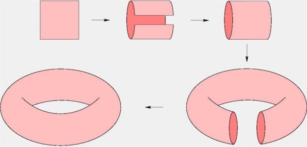
So, what is a quotient topology? Well, the idea is that we will "identify points". More colourfully, we will shrink a whole subset (or whole subsets) to a point (or points). For example: when you take the disk in $\mathbb{R}^2$ and identify all the points of the boundary (the 1-dimensional sphere $S^1$), you get the 2-dimensional sphere $S^2$:










When you take a square, and identify a point of each side with its "opposite", you get a torus.

Ok, so now we go to the theory. (First, let me remark the following: I will assume that the equivalence between a "partition of a set" and "equivalence classes" of some equivalence relation is well-understood. To every partition of a set, we can define the equivalence class: "$x \sim x'$ if $x$ is in the same subset of $x'$". And every equivalence class determines a partition of a set.)

With that in mind, let's begin:

Definition: If $X$ is a topological space and we have a partition of $X$, call $X^*$ the set of those subsets that form the partition. Give $X^*$ the following topology: A subset of $X^*$ (which is a collection of subsets of X) is open if and only if the union of that collection is open in $X$. This is the quotient space.

Equivalently, if $X$ is a topological space and we have an equivalence relation $\sim$, call $X/ \sim$ the quotient space (meaning, the set of equivalence classes). We then have the map: $\pi :X \rightarrow X / \sim$ that takes $x$ to its equivalence class $\bar{x}$. Now, give  $X/ \sim$ the following topology: $U'$ is open in $X/ \sim$ if and only if $\pi^{-1}(U')$ is open in $X$. This is the quotient space.


It may not be easy to see that they are equivalent at a first glance if you are not familiar with equivalence relations, or with topology, but a bit of thought will make it clear. I will adopt the latter definition in the calculations (but will write $X/ \sim $ as $X^*$ for convenience) since it is more algebraic, hence, easier to handle.

Now, before introducing the next useful theorem, let me give some acquaintance to commutative diagrams. Consider the isomorphism theorem:

Isomorphism Theorem: Given an homomorphism $f: G \rightarrow H$ between two groups, we have $\displaystyle G/\ker(f) \simeq Im(\phi)$.

What this theorem says can be given more precision, in the following language:

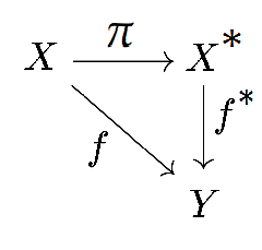
Isomorphism Theorem: Every homomorphism $f: G \rightarrow H$ between two groups induces an injective homomorphism $\bar{f}: G / \ker(\phi) \rightarrow H$  making the following diagram commute (meaning: $f= \bar{f} o \pi$) 











Take a minute to understand this and then we can proceed:


Proposition: Given $X, Y$ topological spaces, a continuous $f:X\rightarrow Y$ which is constant on every equivalence class induces a continuous map $f^*: X^* \rightarrow Y$ making the following diagram commute:

Demonstration: Well, recall the proof of the isomorphism theorem: what happens is that, when you define the map, you must show that it independs of the representative of the class for it to be well-defined. In that case, that happens because the quotient is on the kernel. In this case, it is even simpler: $f$ is constant in the equivalence class!
Define $f^*(\bar{x})=f(x)$. It is well-defined by the previous observation, and obviously $f=f^*o\pi$. It remains to show that $f^*$ is continuous. Lets show pre-image of open is open! But, a set $U$ is open in $X^*$ if and only if $\pi^{-1} U$ is open in $X$. So, we have to show that, for every open $V$ in $Y$, $\pi^{-1} o f^{*-1} (V)$ is open. But this set is exactly $f^{-1}(V)$. Since $f$ is continuous, we have proved $f^*$ is continuous.

Let's see an application of this and prove... that the circle is a segment where you identify the endpoints!







Consider $I:=[0,2\pi]$, and $S^1:=(\cos(t),\sin(t))$, for $t \in [0,2\pi)$. Now, make the following equivalence relation in $I$: every point is equivalent only to itself, except $0$ and $2\pi$, which are equivalent (they are in the same equivalence class). Therefore, we have $I^*$

Take the map $f: I \rightarrow S^1$ that takes $x$ to $(\cos(x), \sin(x))$. Note that $f(0)=f(1)$. So, $f$ satisfies the hypothesis of our preceding proposition (namely, it is constant in every class!). Then, we have an induced continuous map $f^*: I^* \rightarrow S^1$. (Note that $f^*$ is bijective). Now, take the following map: $g: S^1 \rightarrow I^* $ that takes $(\cos(x), \sin(x))$ to $\bar{x}$). It is obviously continuous on all points, except possibly at $f(1,0)$ (since all other classes are points). But the neighbourhoods of $f^*(1,0)=\bar{1}=\bar{0}$, now that we are at the quotient space, must "contain" a neighbourhood of $1$ and a neighbourhood of $0$. Why? Suppose you have a neighbourhood $\bar{U}$ of $\bar{1}$. So, $\pi^{-1}(\bar{U})$ must be an open set containing $0$ and $1$. Therefore, there are two small intervals around $0$ and $1$ in $\pi^{-1}(\bar{U})$, which will be taken to the corresponding classes. So, this $g$ is continuous, since we can take a small enough piece of the circle around $(1,0)$ for which the function will fall inside those intervals. But this $g$ is the inverse of $f^*$. So, we found a homeomorphism. We could also do something more elegant (but would need more knowledge about topology): Since $I$ is compact, so is $I^*$. But $f^*$ is bijective, and $S^1$ hausdorff, so $f^*$ is in fact a homeomorphism.

In Pt.3, we shall talk about another style of glueing things.